Averages, Range, Interquartile Measures, and Boxplots
In addition to the length of a particular work, it can also be useful to know something about the general characteristics of a work such as the average length of a Greek tragedy. The average - or arithmeitc mean - is calculated by taking the sum of the items in a list and dividing it by the number of items in the list. For example, to calculate the average length of a play written by Aeschylus, we would add up the number of words in each play and divide by seven. In R, we complete this calculation with the command mean(). To calculate the mean length of Aeschylus' plays, use the command mean(trag.length[trag.length$Author=="Aeschylus", "Word.Count"]) to get the result of 5728.143. or the command mean(trag.length[trag.length$Author=="Sophocles", "Word.Count"]) to get the result of 8521.5714 for Sophocles' plays.
It is important to realize that the mean value can be extremely misleading depending on the nature of our underlying data. If, for example, the mean of the list of numbers 1, 1, 1, 1, 1, 1, 1, 1000 is 125.875 - a number that bears very little relationship to any of the actual values in the list. Statisticians also use other metrics that help characterize the distribution of values in a data-set including the range, the median value, and the interquartile range.
The range provides one extremely useful set of information about the dataset. It consists of the minimum value and the maximum value in a list. For our extremely simple dataset in the previous chapter, the minimum value would be 1 and the maximum value would be 1000. Both numbers can be calculated using the R command range. If you are only interested in one value, they can be calculated using the R commands min and max.
The median value is quite simply the mid-point of a set where half of the values will be larger than the medium and the other half will be smaller. For a small data set with an odd number of values, the median can be determined by arranging the set in numeric order and then taking the middle value. For example, the length of Sophocles' seven plays in ascending order are: 7177 7363 7914 8702 8830 9280 10385. The median value of this list is 8702; half of Sophocles' plays are longer than this and half are shorter. ((Kenny(1982) pp. 37-39 describes the equation used to calculate the median value for a large data set.)) The R command to determine the median value for Sophocles' plays is median(trag.length[trag.length$Author=="Sophocles", "Word.Count"]).
A measure that is similar to the median value is the interquartile range for a data set. Whereas the median gives the value at the midpoint in a data set where half the values are smaller and half are larger, the interquartile range provides similar numbers for 25%, 50% and 75% of the items in the list respectively. For example, the value of the first quartile is the number where 25% of the values are smaller and 75% are larger. ((Kenny(1982) pp. 58-59 describes the equation used to calculate quartlies.)) This is calculated using the R command quantile. Using our small Sophocles dataset again, we can issue the command quantile(trag.length[trag.length$Author=="Sophocles", "Word.Count"]) and get the result:
| 0% | 25% | 50% | 75% | 100% |
| 7177.0 | 7638.5 | 8702.0 | 9055.0 | 10385.0 |
summary(). The command summary(trag.length[trag.length$Author=="Sophocles", "Word.Count"]) gives us the output
| Min. | 1st Qu. | Median | Mean | 3rd Qu. | Max. |
| 7177 | 7638 | 8702 | 8522 | 9055 | 10380 |
If used with the summary command is used in conjunction with the tapply function described previously, we can quickly compare the characteristics of the tragedies written by Sophocles, Aeschylus, and Eurpidies. tapply(trag.length[, "Word.Count"], trag.length[, "Author"], summary)
| Author | Min. | 1st Qu. | Median | Mean | 3rd Qu. | Max. |
| Aeschylus | 4939 | 5152 | 5297 | 5728 | 5685 | 8187 |
| Sophocles | 7177 | 7638 | 8702 | 8522 | 9055 | 10380 |
| Euripides | 4104 | 7128 | 7787 | 7799 | 9029 | 10030 |
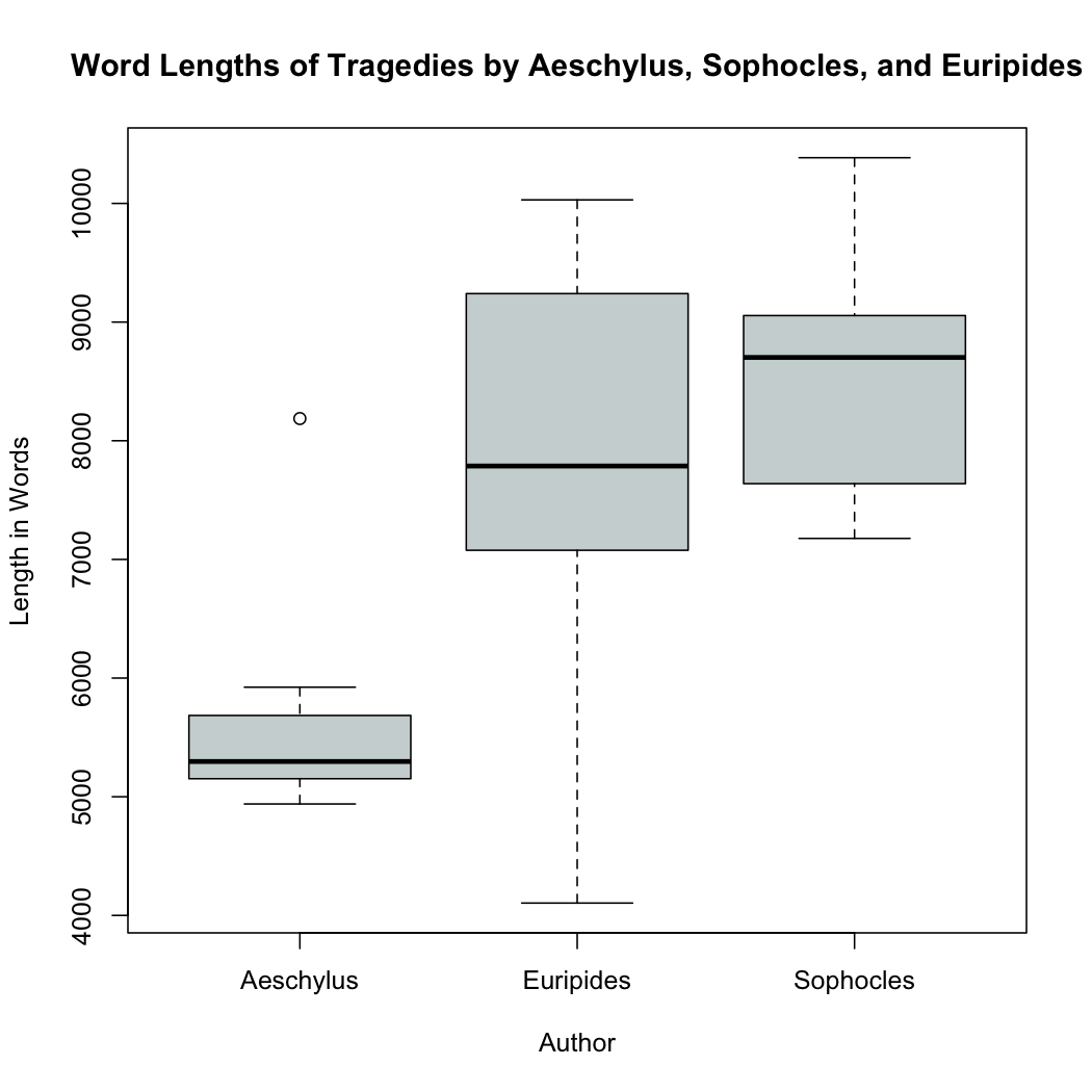
The R graphics library also includes a command to generate a boxplot that concisely presents all of this data in a visual form. The command to generate this graph is boxplot(trag.length[, "Word.Count"] ~ trag.length[, "Author"], main="Word Lengths of Tragedies by Aeschylus, Sophocles, and Euripides", ylab="Length in Words", xlab="Author", col=(c("azure3"))) This command has the same basic structure as other commands we have used but with a few more options.  The first part of the command --
 trag.length[, "Word.Count"] ~ trag.length[, "Author"] -- is the data we want to graph. This formula tells the boxplot command to graph the word lengths of each tragedy summarized by author. Everything after this defines formatting for the chart; xlab is the label for the x-axis, ylab is the label for the y-axis, and the col command defines the color of the plotted rectangle.
The boxplot presents the interquartile range from 25% to 75% as a rectangle on the chart. The mean for the data set is plotted as a solid black line across the rectangle while the range is plotted with dotted lines extending from the central rectangle up to the maximum and down to the minimum. This graph shown to the right allows us easily see that on average Aeschylus' plays are shorter than those by Sophocles and Euripides. We can also see that Aeschylus' plays fall within a much smaller range than vary and that their length varies substantially less than those of Euripides or Sophocles.
<<-- Previous: Graphing Results: Bar Graphs and Pie Charts
Histograms -->>